The purpose of this project is to have the student become familiar with the topic of microwave remote sensing of column water vapor (W) and cloud liquid water path (L). These quantities are derived starting with the radiative transfer equation for a nonscattering atmosphere and arriving at the equations used by Greenwald et al. JGR 98, No.D10, pp 18471-18488, 1993. (You will need to get this reference!) Results of this physical retrieval are to be compared to the results found by the Frank Wentz's all-weather retrieval, JGR 102, No. C4, pp 8703-8718, also available here. This is also sometimes called the "Remote Sensing Systems" (RSS) retrieval. 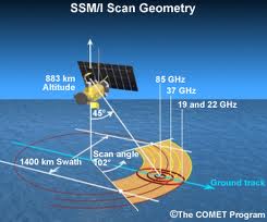The data to be used in this project will be described in more detail shortly and will include SSM/I microwave brightness temperatures. The SSM/I makes observations at four frequencies in the microwave region (19.35, 22.235, 37.0, 85.5 GHz). Horizontal and vertical polarization measurements are made at 19.35, 37.0, and 85.5 GHz while 22.235 GHz has only vertical polarization measurements. Only the 19.35, 22.235, and 37.0 GHz data are provided in gridded, average form in the file ssmi_jan90.txt

1. The integral form of the radiative transfer equation for brightness temperatures under the Rayleigh-Jeans approximation for a satellite at the top-of-atmosphere (TOA) looking down is as follows:
   
   where T_s is the surface temperture, T_cmb is the temperature of cold space, T(τ) is the atmospheric profile, μ is the cosine of the viewing zenith angle, and τ is the optical depth vertical coordinate taken from the TOA. τ* denotes the surface-to-space total optical depth, and R^P is the surface reflectivity for a given polarization state P, where P is either vertical (V) or horizontal (H) polarization. Note that this is essentially equation 7.21 in Chapter 7 of Stephens, with some mistakes corrected.
   
   First explain what each of the four terms correspond to. Then, using this relation, show that the brightness temperature (TB) received by a satellite viewing an isothermal atmosphere at microwave frequencies can be approximated by
   
   where t* is the surface-to-space transmission at a given frequency for this view angle. Be sure to show all steps. This equation is useful when atmospheric emission is coming primarily from near the surface, as for water vapor and low clouds.

2. Derive eqn (7.25) in Chapter 7 of Stephens given the preceding relationship.

3. Using the method of Greenwald et al. (1993), produce global maps of monthly precipitable water (== column water vapor, referred to as CWV or W) and cloud liquid water (== liquid water path, referred to as LWP or L) for January 1990. In practice we usually carry out the retrievals on the pixel level and then grid and average the data accordingly. This is impractical for this exercise. To save time, the brightness temperature data have been gridded and averaged to produce monthly mean fields. The retrieval of precipitable water and cloud liquid water is then applied to these data. After creating the global maps of column water vapor and liquid water path, compute the zonally-averaged values for each quantity. Given knowledge of the basic general circulation of our planet, identify features which show both low and high values of precipitable water and cloud liquid water. How do you think these maps and figures would change for July 1990? Perform the retrieval again for July 1990 and comment on the results. Be sure to show units in all plots.

4. Compare the results given by this simple retrieval with the results from the Remote Sensing Systems physical retrieval, a well-established and fairly standard retrieval (RSS water vapor retrievals are pretty much considered the current standard in the field). This method simultaneously retrives surface wind speed, column water vapor, column liquid water and rain rate by using all SSM/I channels except the 85 GHz channels. Comment on any large differences between the results of the two retrievals in any of the retrieved variables (wind speed, water vapor, and cloud liquid water). The data files ssmi_jan90.txt and ssmi_jul90.txt already contain the RSS retrieval results, you simply have to read them in. All RSS retrievals can also be obtained from http://www.remss.com.

5. Think about and then comment on the advantages and disadvantages of the Greenwald et al. retrieval as compared to an optimal estimation-style retrieval.

1. The data file ssmi_jan90.txt contains lat, lon, sea surface temperatures from the Reynolds Optimal Interpolation product, and SSM/I brightnes temperatures (TB) on a 360x180 1 degree lat/lon grid. These values have been averaged over the month of January 1990 and down to the 1-degree scale. The file ssmi_jul90.txt similarly contains values for July of 1990.

2. It should be noted that all values of 999.99 in the brightness temperature data are areas of land, ice, or non oceanic areas which should be treated as missing values. The SST data do not have corresponding missing values, so the brightness temperature data should be used as a template to remove the areas of ``missing'' data. Also, areas north of 80N and south of 80S have been removed and replaced with values 999.99 since little information concerning water vapor can be extracted from the microwave in these regions.

3. It is left to each individual to figure out ways of displaying the data.

1. In addition to the data, two subroutines are supplied to assist in the retrievals. You will also need to retrieve the surface wind speed in order to derive the surface emissitivity and hence surface reflectivity. For this purpose, we employ the statistical model of Goodberlet et al. (1989) which is simple. [The student should consult this reference to see how well the retrieval works compared to actual surface wind data]. This retrieval reduces to
   
   SPEED=1.0969(T19V) - 0.4555(T22V) - 1.76(T37V) + 0.786(T37H) + 147.9
   
   where SPEED is the wind speed in meters per second. A quality control check to ensure the wind speed is $>0$ is recommended. It should be noted that the method of Gooberlet doesn't work as well in the tropics, but its deficiencies will be ignored for the purposes of this project.

2. Once the wind speed is established, the surface emissivity is derived from the subroutine EMISS provided in file emiss.f (or emiss.pro) The water vapor and liquid water absorption coefficients as well as the oxygen transmission are provided in the subroutine COEF in file coef.f (coef.pro). This requires the SST as input. The view angle of the SSM/I satellite (F8) is approximately 53.1 degrees.

3. To perform the retrieval, you will need values at 19.35 and 37.0 GHz for the transmittance due to oxygen, the volume absorption coefficient of water vapor, and the volume absorption coefficient of cloud liquid water, all as a function of temperature. The routine coef.f (or coef.pro) does this for you. It makes the same assumptions as Greenwald regarding the temperature dependence of each, and specifically assumes that the water vapor is largely at the surface temperature, and the liquid cloud is 6 deg C. colder than the surface.

4. The method of Greenwald et al. (1993) is simply a recasting of eqn (7.25), in which the quantity (R_V - R_H) is replaced with R_V*(1-F), where F is defined to be
   
   F = (TB_H - Tbar) / (TB_V - Tbar)
   
   Greenwald takes Tbar=Ts-3.58 at 37 GHz. The value of 3.58 was used to tune the retrieval and should not be regarded as having a real physical meaning. At 19.35 GHz, Tbar is initially assumed to equal the surface temperature Ts. This is used to retrieve initial values of W and L. If the initial W > 25 kg/m^2, you are to iterate using equations (2) and (4) from Greenwald et al. (1993) until a stable value of W is obtained. Convergence is obtained when abs(W_new - W_old) < 0.1 kg/m^2. Convergence should generally occur after 2 to 3 iterations. Ignore any W retrievals with values exceeding 100 kg/m^2.

5. When you apply equations (7) and (8) from Greenwald et al., you will occasionally get negative values for W and/or L. Be sure to set these values to zero in order to be physical. Note that sometimes retrievals will actually allow the negative values to remain, as forcing them to zero will bias statistical averages. But in this case, leaving the negative values can screw up the iterative process, so we take the safe road and set them to zero.

• readme.first
• ssmi_jan90.txt
• ssmi_jul90.txt
• emiss.f OR emiss.pro
• coef.f OR coef.pro

1. This project uses monthly averaged brightness temperatures while Greenwald's retrieval computed the W and L values at each pixel and averaged those values over each month.

2. The monthly averaged brightness temperatures used in this project include pixels in precipitating regions. This results in overestimating the W and L values, particularly in regions of persistent precipitation (ie. the ITCZ and the midlatitude storm tracks).

3. This project uses a newer parameterization of ocean surface emissivity that is based on the UK Met Office FASTEM-2 algorithm.

4. The surface wind speed algorithm in Greenwald et al. (1993) differed for regions where the SST exceeded 300K. Greenwald et al. (1993) explains that Goodberlet's method produces erroneously high values in the tropical regions, thus the method of Bates (1991, Jour. Geophys. Res.) was used in those regions. This results in increasing the CWV and decrease the LWP in these regions.

For the July 1990 data, the first useable brightness temperature data occurs at Lat=-64.5, Lon=180.5. Here some values your TA computed for this point using the routines given.

1. SST = 271.35 K
2. SSM/I Tb's (19H,19V,22H,37H,37V) = 113.57, 183.24, 194.80, 148.13, 208.11
3. wind speed = 10.32 m/s
4. emissivities (19H,19V,37H,37V) = 0.3136, 0.6142, 0.3799, 0.6996
5. abs. coeffs. (kl19,kl37,kv19,kv37) = 0.09949, 0.32577, 0.00271, 0.00212
6. O2 Trans (19,37) = 0.97804, 0.92711
7. F19, F37 = 1.79072, 2.00536
8. τ₁, τ₂ = 0.038414, 0.048228
9. CWV (W) = 11.5029 kg/m^2
10. CLW (L) = 0.07319 kg/m^2

Below are values for Lat=1.5, Lon=0.5, also in July 1990. This one requires iteration as the initial water vapor path is greater than 25 kg/m²

1. SST = 298.35 K
2. SSM/I Tb's (19H,19V,22H,37H,37V) = 152.66, 210.12, 245.0, 170.43, 223.48
3. wind speed = 7.42 m/s
4. emissivities (19H,19V,37H,37V) = 0.2737, 0.5652, 0.3089, 0.6153
5. abs. coeffs. (kl19,kl37,kv19,kv37) = 0.0477, 0.1686, 0.00259, 0.00212
6. O2 Trans (19,37) = 0.9796, 0.9330
7. F19, F37 = 1.651, 1.744 (first iteration), = 1.663, 1.744 (final value)
8. τ₁, τ₂ = 0.10337, 0.10134 (first iteration), = 0.10864, 0.10134 (final values)
9. CWV (W) = 37.60 kg/m^2 (first iteration), 40.25 kg/m^2 (final value)
10. CLW (L) = 0.1283 kg/m^2 (first iteration), 0.0950 kg/m^2 (final value)